59 11.6 Non-Ideal Gas Behavior
Learning Objectives
By the end of this section, you will be able to:
- Describe the physical factors that lead to deviations from ideal gas behavior
- Explain how these factors are represented in the van der Waals equation
- Define compressibility (Z) and describe how its variation with pressure reflects non-ideal behavior
- Quantify non-ideal behavior by comparing computations of gas properties using the ideal gas law and the van der Waals equation
Thus far, the ideal gas law, PV = nRT, has been applied to a variety of different types of problems, ranging from reaction stoichiometry and empirical and molecular formula problems to determining the density and molar mass of a gas. As mentioned in the previous modules of this chapter, however, the behavior of a gas is often non-ideal, meaning that the observed relationships between its pressure, volume, and temperature are not accurately described by the gas laws. In this section, the reasons for these deviations from ideal gas behavior are considered.
One way in which the accuracy of PV = nRT can be judged is by comparing the actual volume of 1 mole of gas (its molar volume, Vm) to the molar volume of an ideal gas at the same temperature and pressure. This ratio is called the compressibility factor (Z) with:
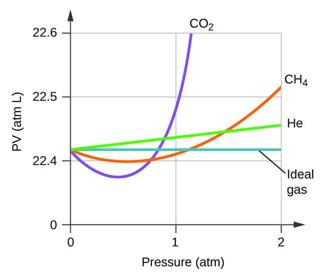
Ideal gas behavior is therefore indicated when this ratio is equal to 1, and any deviation from 1 is an indication of non-ideal behavior. Figure 1 shows plots of Z over a large pressure range for several common gases.
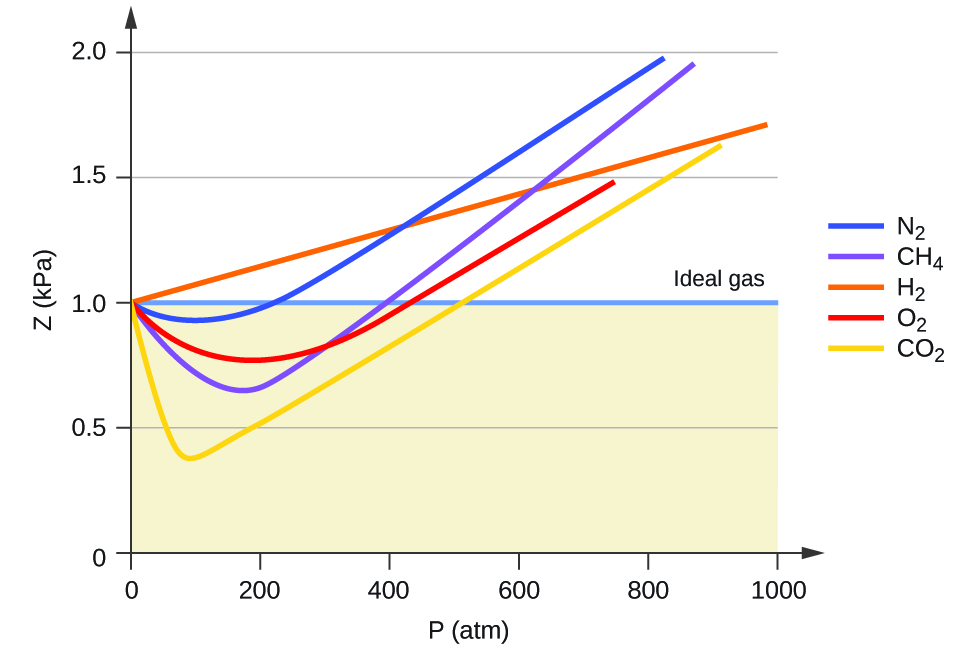
As is apparent from Figure 1, the ideal gas law does not describe gas behavior well at relatively high pressures. To determine why this is, consider the differences between real gas properties and what is expected of a hypothetical ideal gas.
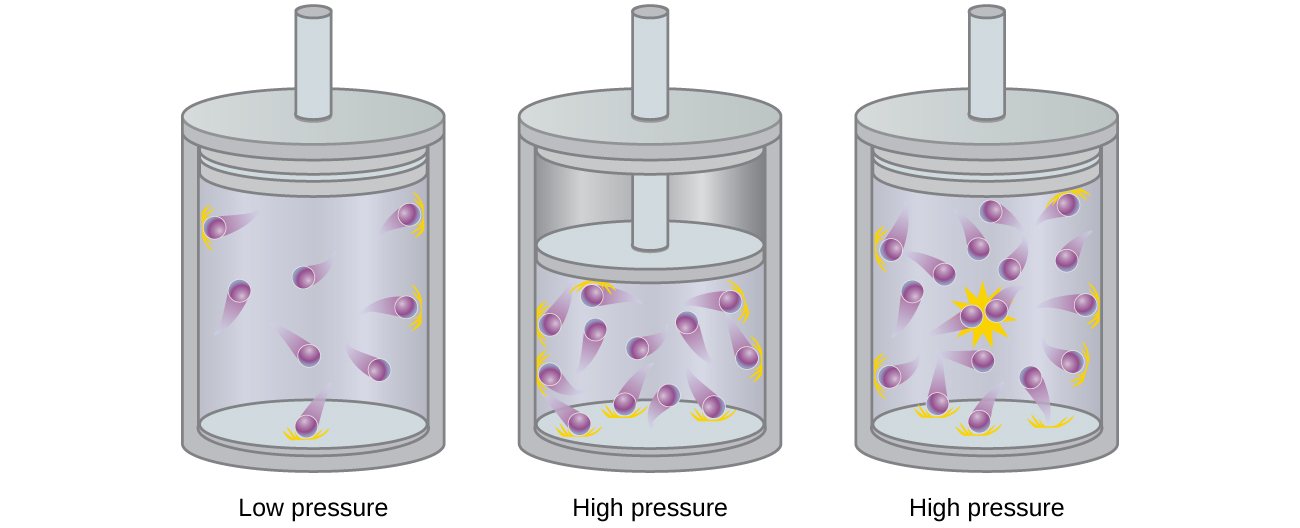
Particles of a hypothetical ideal gas have no significant volume and do not attract or repel each other. In general, real gases approximate this behavior at relatively low pressures and high temperatures. However, at high pressures, the molecules of a gas are crowded closer together, and the amount of empty space between the molecules is reduced. At these higher pressures, the volume of the gas molecules themselves becomes appreciable relative to the total volume occupied by the gas (Figure 2). The gas therefore becomes less compressible at these high pressures, and although its volume continues to decrease with increasing pressure, this decrease is not proportional as predicted by Boyle’s law.
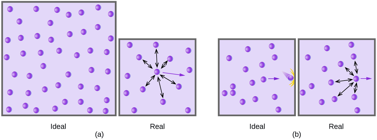
At relatively low pressures, gas molecules have practically no attraction for one another because they are (on average) so far apart, and they behave almost like particles of an ideal gas. At higher pressures, however, the force of attraction is also no longer insignificant. This force pulls the molecules a little closer together, slightly decreasing the pressure (if the volume is constant) or decreasing the volume (at constant pressure) (Figure 3). This change is more pronounced at low temperatures because the molecules have lower KE relative to the attractive forces, and so they are less effective in overcoming these attractions after colliding with one another.
There are several different equations that better approximate gas behavior than does the ideal gas law. The first, and simplest, of these was developed by the Dutch scientist Johannes van der Waals in 1879. The van der Waals equation improves upon the ideal gas law by adding two terms: one to account for the volume of the gas molecules and another for the attractive forces between them.
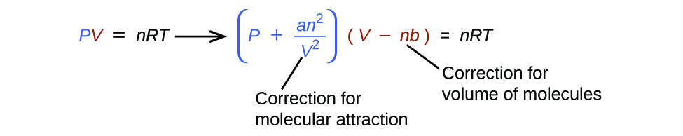
The constant a corresponds to the strength of the attraction between molecules of a particular gas, and the constant b corresponds to the size of the molecules of a particular gas. The “correction” to the pressure term in the ideal gas law is [latex]\frac{n^2a}{V^2}[/latex], and the “correction” to the volume is nb. Note that when V is relatively large and n is relatively small, both of these correction terms become negligible, and the van der Waals equation reduces to the ideal gas law, PV = nRT. Such a condition corresponds to a gas in which a relatively low number of molecules is occupying a relatively large volume, that is, a gas at a relatively low pressure. Experimental values for the van der Waals constants of some common gases are given in Table 3.
| Gas | a (L2 atm/mol2) | b (L/mol) |
|---|---|---|
| N2 | 1.39 | 0.0391 |
| O2 | 1.36 | 0.0318 |
| CO2 | 3.59 | 0.0427 |
| H2O | 5.46 | 0.0305 |
| He | 0.0342 | 0.0237 |
| CCl4 | 20.4 | 0.1383 |
| Table 3. Values of van der Waals Constants for Some Common Gases | ||
At low pressures, the correction for intermolecular attraction, a, is more important than the one for molecular volume, b. At high pressures and small volumes, the correction for the volume of the molecules becomes important because the molecules themselves are incompressible and constitute an appreciable fraction of the total volume. At some intermediate pressure, the two corrections have opposing influences and the gas appears to follow the relationship given by PV = nRT over a small range of pressures. This behavior is reflected by the “dips” in several of the compressibility curves shown in Figure 1. The attractive force between molecules initially makes the gas more compressible than an ideal gas, as pressure is raised (Z decreases with increasing P). At very high pressures, the gas becomes less compressible (Z increases with P), as the gas molecules begin to occupy an increasingly significant fraction of the total gas volume.
Strictly speaking, the ideal gas equation functions well when intermolecular attractions between gas molecules are negligible and the gas molecules themselves do not occupy an appreciable part of the whole volume. These criteria are satisfied under conditions of low pressure and high temperature. Under such conditions, the gas is said to behave ideally, and deviations from the gas laws are small enough that they may be disregarded—this is, however, very often not the case.
Example 1
Comparison of Ideal Gas Law and van der Waals Equation
A 4.25-L flask contains 3.46 mol CO2 at 229 °C. Calculate the pressure of this sample of CO2:
(a) from the ideal gas law
(b) from the van der Waals equation
(c) Explain the reason(s) for the difference.
Solution
(a) From the ideal gas law:
(b) The van der Waals equation:
This finally yields P = 32.4 atm.
(c) This is not very different from the value from the ideal gas law because the pressure is not very high and the temperature is not very low. The value is somewhat different because CO2 molecules do have some volume and attractions between molecules, and the ideal gas law assumes they do not have volume or attractions.
Check your Learning
A 560-mL flask contains 21.3 g N2 at 145 °C. Calculate the pressure of N2:
(a) from the ideal gas law
(b) from the van der Waals equation
(c) Explain the reason(s) for the difference.
Answer:
(a) 46.562 atm; (b) 46.594 atm; (c) The van der Waals equation takes into account the volume of the gas molecules themselves as well as intermolecular attractions.
Key Concepts and Summary
Gas molecules possess a finite volume and experience forces of attraction for one another. Consequently, gas behavior is not necessarily described well by the ideal gas law. Under conditions of low pressure and high temperature, these factors are negligible, the ideal gas equation is an accurate description of gas behavior, and the gas is said to exhibit ideal behavior. However, at lower temperatures and higher pressures, corrections for molecular volume and molecular attractions are required to account for finite molecular size and attractive forces. The van der Waals equation is a modified version of the ideal gas law that can be used to account for the non-ideal behavior of gases under these conditions.
Key Equations
- [latex]\text{Z} = \frac{\text{molar volume of gas at same} \;T \;\text{and} \;P}{\text{molar volume of ideal gas at same} \;T \;\text{and} \;P} = (\frac{P \times V_m}{R \times T})_{\text{measured}}\\[0.5em][/latex]
- [latex](P + \frac{n^2a}{V^2}) \times (V - nb) = nRT[/latex]
Chemistry End of Chapter Exercises
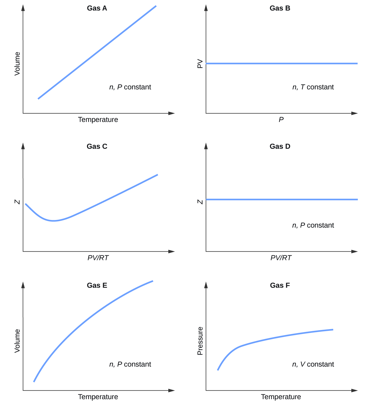
- Graphs showing the behavior of several different gases follow. Which of these gases exhibit behavior significantly different from that expected for ideal gases?
- Explain why the plot of PV for CO2 differs from that of an ideal gas.
- Under which of the following sets of conditions does a real gas behave most like an ideal gas, and for which conditions is a real gas expected to deviate from ideal behavior? Explain.
(a) high pressure, small volume
(b) high temperature, low pressure
(c) low temperature, high pressure
- Describe the factors responsible for the deviation of the behavior of real gases from that of an ideal gas.
- For which of the following gases should the correction for the molecular volume be largest:
CO, CO2, H2, He, NH3, SF6?
- A 0.245-L flask contains 0.467 mol CO2 at 159 °C. Calculate the pressure:
(a) using the ideal gas law
(b) using the van der Waals equation
(c) Explain the reason for the difference.
(d) Identify which correction (that for P or V) is dominant and why.
- Answer the following questions:
(a) If XX behaved as an ideal gas, what would its graph of Z vs. P look like?
(b) For most of this chapter, we performed calculations treating gases as ideal. Was this justified?
(c) What is the effect of the volume of gas molecules on Z? Under what conditions is this effect small? When is it large? Explain using an appropriate diagram.
(d) What is the effect of intermolecular attractions on the value of Z? Under what conditions is this effect small? When is it large? Explain using an appropriate diagram.
(e) In general, under what temperature conditions would you expect Z to have the largest deviations from the Z for an ideal gas?
Glossary
- compressibility factor (Z)
- ratio of the experimentally measured molar volume for a gas to its molar volume as computed from the ideal gas equation
- van der Waals equation
- modified version of the ideal gas equation containing additional terms to account for non-ideal gas behavior
Solutions
1. Gases C, E, and F
3. The gas behavior most like an ideal gas will occur under the conditions in (b). Molecules have high speeds and move through greater distances between collision; they also have shorter contact times and interactions are less likely. Deviations occur with the conditions described in (a) and (c). Under conditions of (a), some gases may liquefy. Under conditions of (c), most gases will liquefy.
5. SF6
7. (a) A straight horizontal line at 1.0; (b) When real gases are at low pressures and high temperatures they behave close enough to ideal gases that they are approximated as such, however, in some cases, we see that at a high pressure and temperature, the ideal gas approximation breaks down and is significantly different from the pressure calculated by the ideal gas equation (c) The greater the compressibility, the more the volume matters. At low pressures, the correction factor for intermolecular attractions is more significant, and the effect of the volume of the gas molecules on Z would be a small lowering compressibility. At higher pressures, the effect of the volume of the gas molecules themselves on Z would increase compressibility (see Figure 1) (d) Once again, at low pressures, the effect of intermolecular attractions on Z would be more important than the correction factor for the volume of the gas molecules themselves, though perhaps still small. At higher pressures and low temperatures, the effect of intermolecular attractions would be larger. See Figure 1. (e) low temperatures
